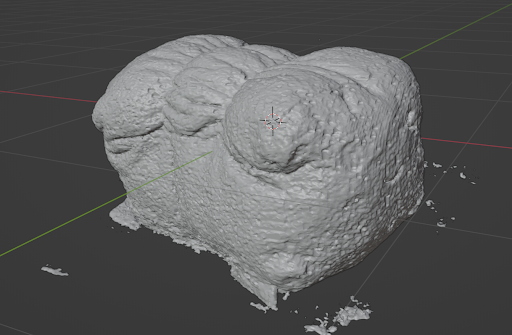
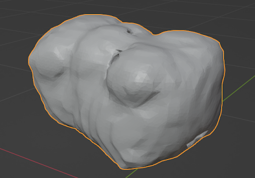
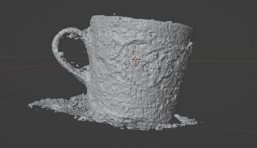
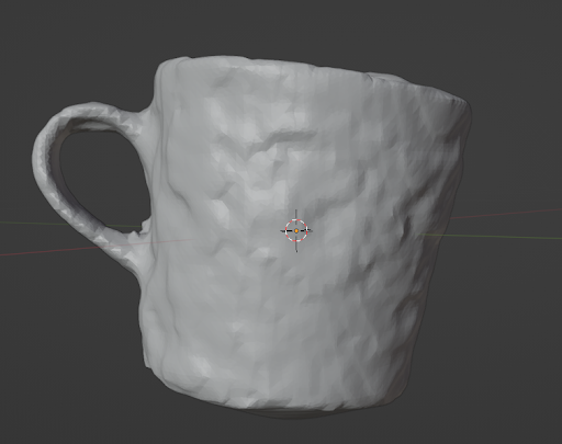
Since its invention in 2020, Neural Radiance Fields (NeRF) has become widely popular in the field of deep learning and computer vision, and it has inspired many papers. Particularly, a team at NVIDIA Research significantly reduced the training cost of the NeRF neural network with their project, Instant Neural Graphics Primitives, or Instant NGP for short. While their paper delivers in speed and accuracy, the 3D meshes generated from their trained model can be noisy. This project aims to improve on Instant NGP’s mesh reconstruction by generating a point cloud of an object from a trained model, cleaning the point cloud with a custom GUI, and feeding the result into a custom pipeline. The pipeline first calculates point cloud normals using PCA(Principal Component Analysis)-based normal estimation then uses the Poisson Surface Reconstruction Algorithm to transform it into a 3D mesh.
|
|
|
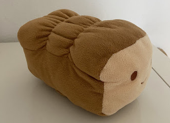
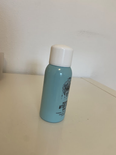
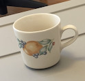
To train an object using Instant NGP, we closely followed the guidelines (linked here) provided by the Instant NGP repository. We began by collecting approximately 100 images of that object at different viewpoints. This was done by capturing a ~1-minute video on an iPhone 11 at 30fps, moving the camera around to capture different perspectives, and sampling at a rate of 2 frames per second. After manually inspecting the images to delete blurry ones, we use COLMAP to extract the camera positions and angles for each image. The resulting images and camera positions were then used to train an Instant NGP model on an NVIDIA Tesla T4 through Google Colab. We used 20,000 training steps and kept all other hyperparameters as default. Each model took around 20 minutes to train, and results were stored in an .ingp binary file.
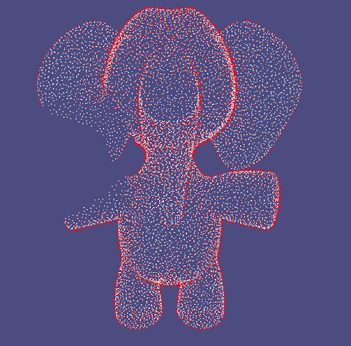
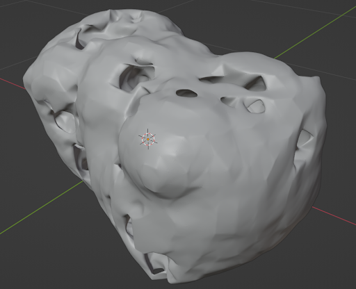
After, we used Instant NGP’s custom GUI to crop the scene so that the bounding box only contained the object of interest. The GUI had a feature to transform the object into a mesh, but it did not have a point cloud option. To remedy this, we wrote code to extract the vertices from Instant NGP’s mesh and exported it as a .ply file using Python’s plyfile package (linked here).
|

|
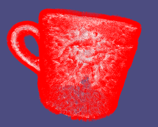
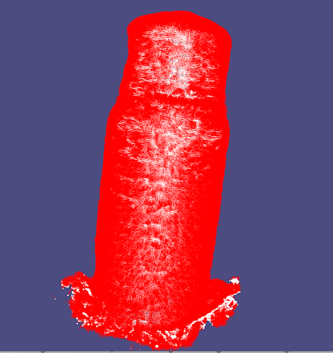
Building a mesh requires the surface normal at each point. Since we can only extract the point clouds vertices themselves, we decided to test three methods to estimate the unoriented normals:
Each of these normal estimation algorithms output two possible normals along the same axis as a result of not knowing the global structure. Therefore, the orientation is adjusted by graph optimization of the Riemannian Graph such that normals are consistent between pairs of tangent planes (which combines both K-Nearest Neighbor and Minimum Spanning Tree to provide approximate correct orientation). We used Open3D’s library in Python for normal estimation and correcting orientation.

|
|
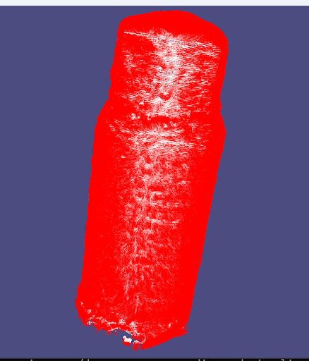
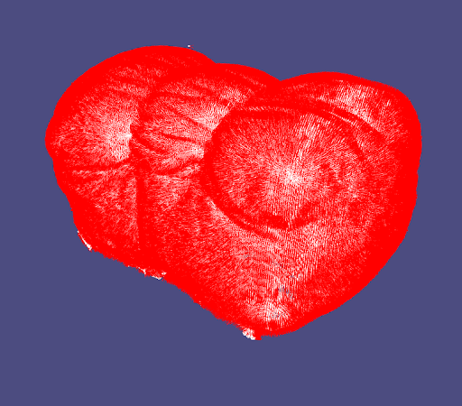
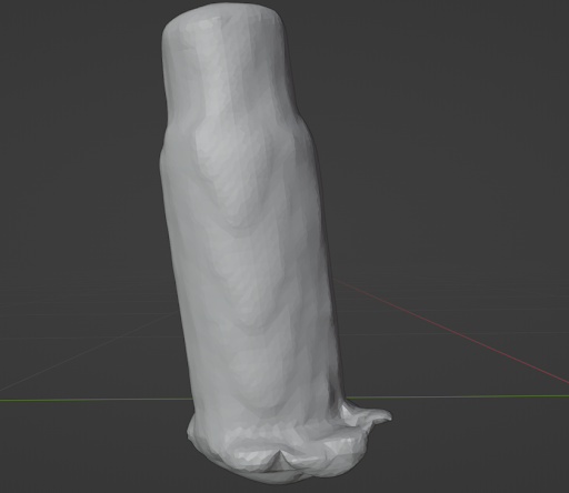
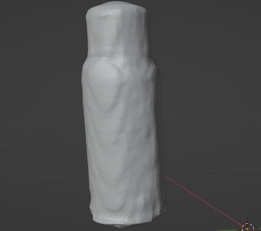
The results of our mesh reconstruction turns out to have higher quality if we clean up the point cloud by removing some of the interior points inside the surface for our pointcloud. Using a plugin from opengl::glfw library, we built a custom UI allowing us to directly clean up the point cloud with a spherical eraser before converting to mesh. We trace the position of the mouse by projecting screen space coordinate to world space coordinate where the point cloud lives in order to decide the position of the eraser.
|
|
|
We obtained our skeleton framework from the University of Toronto, linked here, and used that as a starting point to code the rest of the algorithm from scratch. Given a point cloud and the surface normals of each point, we represent the list of points as a matrix $P$ and the list of normals as a matrix $N$. Additionally, we specify the components of our finite-difference grid that the mesh is rendered within, defining the number of nodes in each dimension ($nx$, $ny$, $nz$), the grid spacing $h$, and the corner $c$ of the finite-difference grid.
First, we construct a sparse matrix $W$ that encodes trilinear interpolation operations between each point and the corresponding voxel (3D box) it lives in. In other words, given the grid nodes of the voxels in a vector $x$, $P = W * x$.
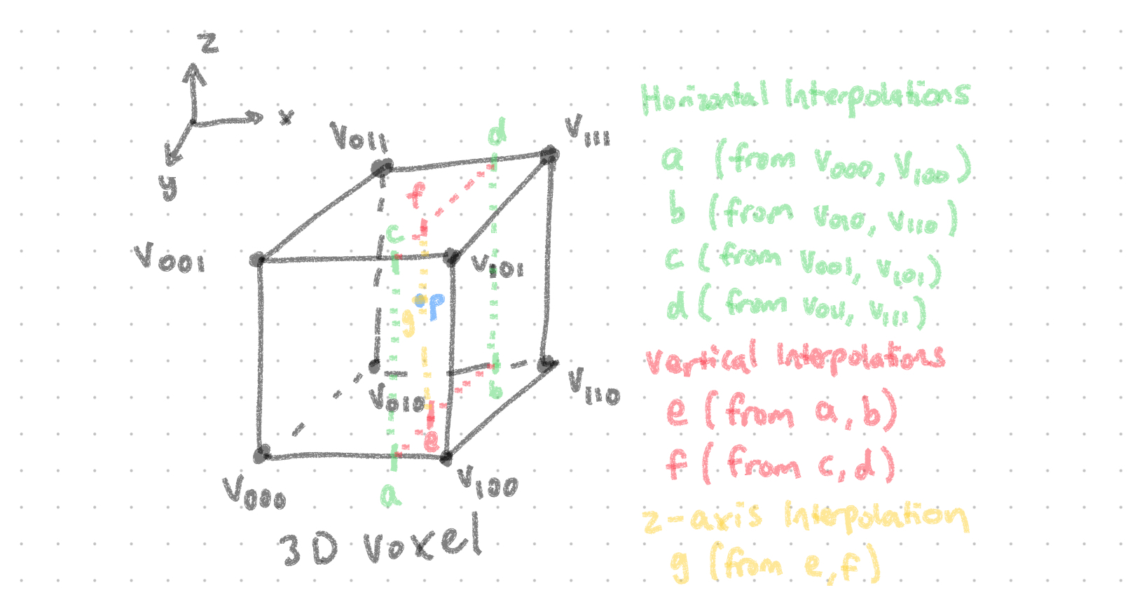
Next, given a voxel $v$ and corresponding point $p$, we can define the trilinear interpolation of $p$ from a series of linear interpolations:
. |
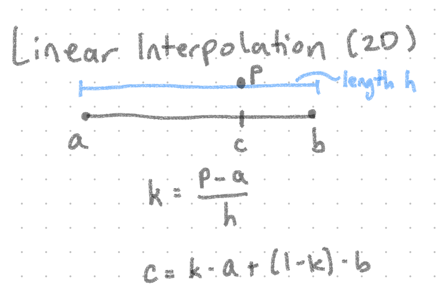
$k$ represents the proportion of $p$ relative to $a$ and $b$ |
When combining all the linear interpolation (lerp) operations for our trilinear operation, we notice the following pattern:
Additionally, we encode each voxel position, $g(i, j, k)$, with the following equation: $i + j * nx + k * nx * ny$. Therefore, for each point $p$ in $P$, we first identify the voxel $p$ belongs to. After, for each corner of the voxel, we set the value $w$ in the matrix $W$ at coordinates $(i, g)$, where $i$ is the index of the current point we are evaluating, $g$ is the encoding of the voxel ID, and $w$ is the corresponding trilinear interpolation weight.
Next, we define a function to construct a sparse matrix $D$ that contains the partial derivatives for a specified direction $dir$ over each point in the finite-difference grid (i.e. we can define three matrices $D_x$, $D_y$, $D_z$). Note that $D$ will encode partial derivatives on a staggered grid that is shifted by 1/2 in the specified $dir$ direction. Logically this makes sense: since we subtract the values of two points to estimate their derivative, we are effectively calculating the derivative in-between both points (i.e. half-way between each one).
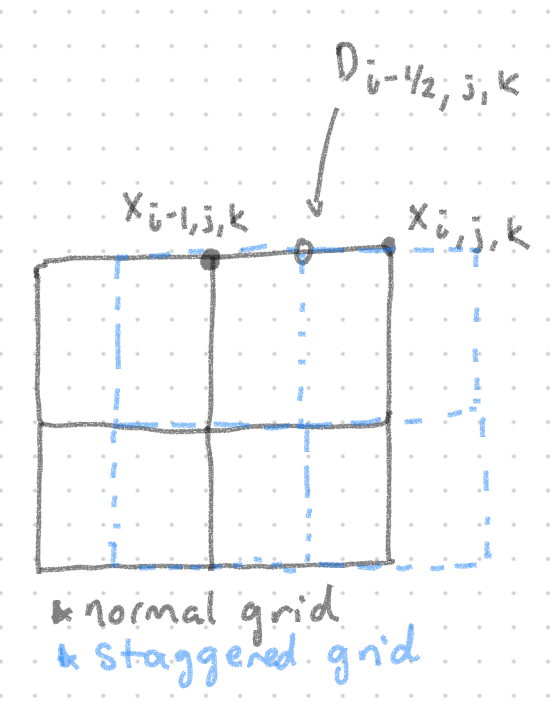
Given the row $D_{i - \frac{1}{2}, j, k}$, we set its corresponding column $c$ to:
Additionally, we encode row $D_{i - \frac{1}{2}, j, k}$ as the value $d = i + j * nx + k * nx * ny$ (this represents the row index in the matrix $D$).
Finally, given our implementation of fd_partial_derivative, we can create the sparse gradient matrix $G$ by concatenating the partial derivative matrices $D_x$, $D_y$, $D_z$ top-to-bottom.
In this function, we construct implicit function $g$ to feed into the Marching Cubes Algorithm to generate a corresponding mesh.
|
|
|
|
|
|
|

|
|
|
|
|
|
|
|
|

|
|
All authors contributed towards brainstorming, designing, implementing, and presenting this project.